Introduction
Introduction to Radio Astronomy, Spectrometers and DESHIMA
- Cosmological formation
- Redshift
- DESHIMA
- Ground-based submillimeter astronomy
- This Project
- Bibliography
The ultimate weapon in the arsenal of a historian just might be a time machine. While historians can infer a lot from written texts and archaeological digs, no substitute can outperform being in the past and observing. Unfortunately for historians, a time machine has yet to be invented. Astronomers, however, are more fortunate in this field.
Around the turn of the century, new physics was being invented to explain previous observations and conclusions. As a result, it was understood that the speed of light was finite and moreover a constant, independent of the speed of the observer, which Albert Einstein postulated in 1905[1]. It logically follows that the arriving light from distant stars and galaxies is reaching us from the past.
Since light is a wave traveling through the expanding universe, it undergoes Doppler shift and therefore cosmological objects that move away from the observer undergo a shift in the frequency of light. This is known as redshift, because the expanding wavelength means that visible light would shift towards the red end of the spectrum. Just 12 years after Einstein's discovery, American Astronomer Vesto Slipher [2] discovered the redshift of distant galaxies and with it cosmological spectroscopy was born.
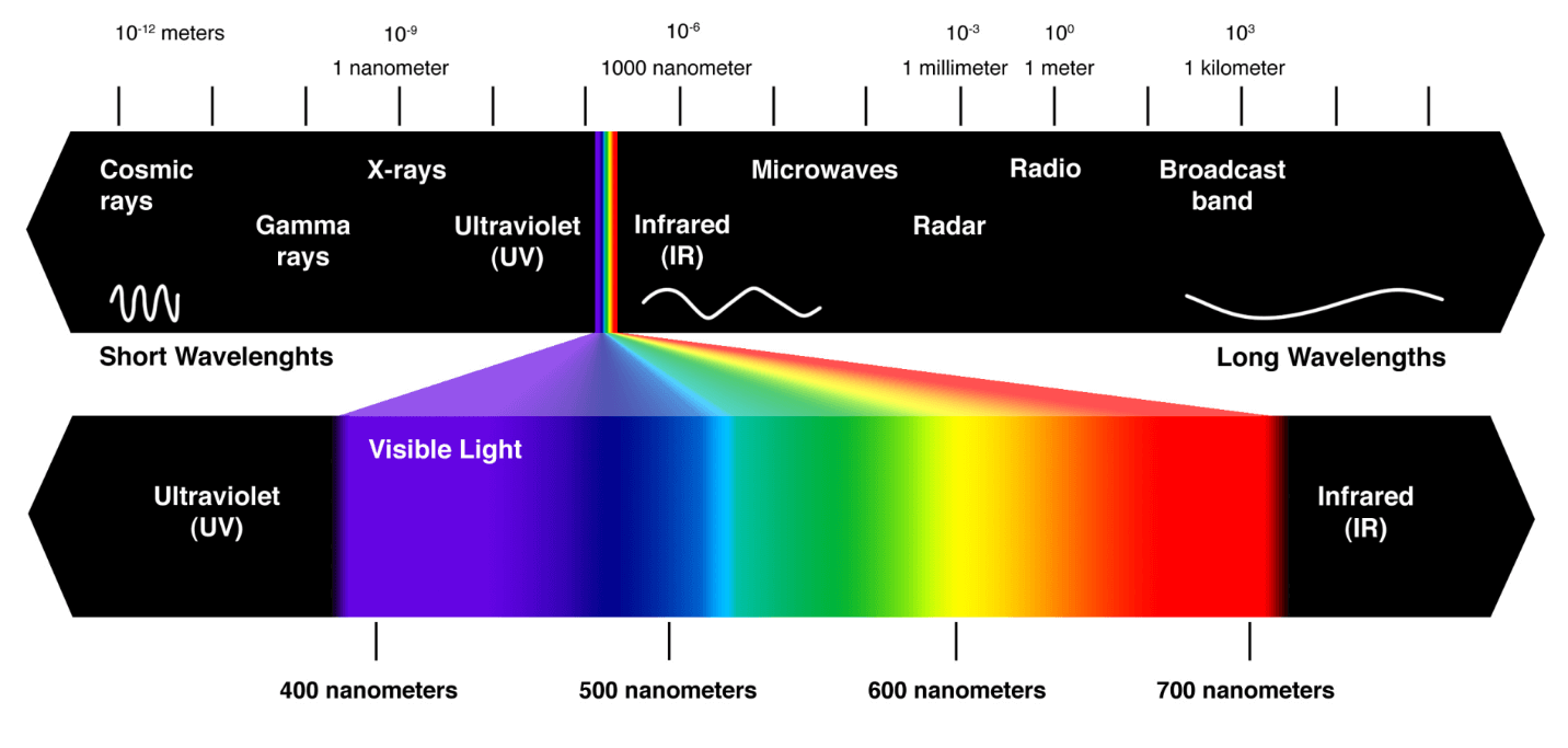
A part of the light spectrum. Visible light is expanded to show the different colors. Note how red light in the visible spectrum has a longer wavelength, giving redshift its name. Image taken from [3]
Combining these effects gives us a sort of astronomical time machine: looking far out into the cosmos means looking into the past where the universe was much younger. However, just pointing a telescope at the night sky poses a few problems.
Cosmological formation
Understanding how stars and galaxies form out of a uniformly gaseous universe is one of the largest areas of research in modern physical cosmology. The physical processes by which these happen might be well understood, but the amount of possible initial values of these processes are so vast that they can have wildly different outcomes[4]. Looking at these events occurring in the distant universe (and therefore distant past) is therefore important to further the understanding of the forming of the universe.
Unfortunately, much of the formation of these cosmological bodies happens inside thick dust clouds which are opaque to visible light and are therefore investigated using what is called sub-millimeter astronomy: astronomy ranging from $100\:\mathrm{\mu m}$ to about $1\:\mathrm{mm}$. In frequency terms, following
$$\begin{equation} f = \frac{c}{\lambda} \end{equation}$$this corresponds with about $150\:\mathrm{GHz}$ to $1500\:\mathrm{GHz}$.
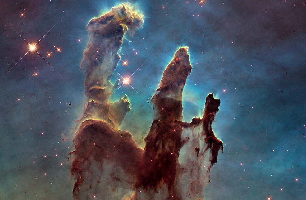 The Messer-16 nebula, dubbed "The Eagle", captured by the Hubble Space Telescope is an example of a dust cloud that is opaque to visible light. Image taken from [5]
Redshift
As mentioned before, the redshift of light gives us the opportunity to calculate the relative speed and therefore distance and age of astronomical sources. By the term "redshift", I mean the following formal definition [6]
$$\begin{equation} 1+z = \frac{f_\mathrm{emit}}{f_\mathrm{obs}} \end{equation}$$where $z$ denotes redshift and $f_\mathrm{emit}$ and $f_\mathrm{obs}$ denote the emitted and observed frequency of a signal respectively. In order to calculate redshift we therefore need to know both frequencies.
Emitted frequency
Quantum mechanics tells us that the electron configuration in atoms exist in quantized states. That is to say: they can move between defined states, but not in the continuum inbetween. When an atom moves from one configuration to a higher state energy is absorbed, when it moves to a lower state energy is emitted. These quantized energy states give way to what is known as spectral lines, where a specific wavelength is known to be emitted by specific atoms.
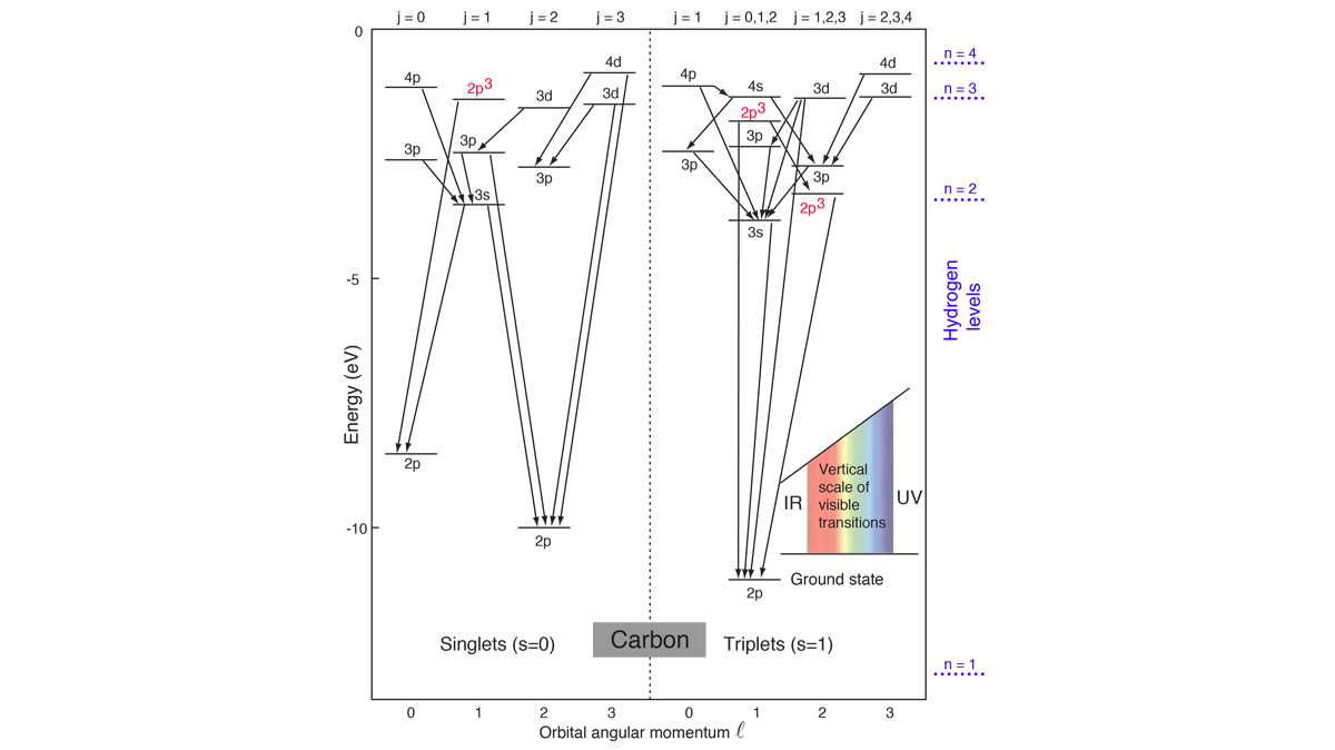 A few energy states of carbon. Note how higher energy gaps result in shorter wavelengths. Image taken from [7]
The energy gaps shown are to wide to emit photons in the submillimeter wavelength range DESHIMA operates in, however fine structure spectral lines are in the correct wavelength gap. This is the splitting of two similar states due to spin and relativistic effects. Another mechanism by which molecules emit spectral lines is due to the shifting in quantized rotational states. The various states astronomical sources split between are well known and therefore can be tracked to measure redshift.
This becomes clear when we look at the spectral flux density $E_{e,\nu}$ of a galaxy, simulated with the Python module galspec[8].
The spectral flux density of a simulated galaxy with different redshifts. Here the spectral flux is given in units of Jansky, which is equivalent to 10-26 WM-2Hz-1
From the figure it is clear that with higher $z$ the peaks move further to the left, towards lower frequencies and therefore longer wavelengths. If one were to look for peaks in incoming signal and measure the wavelength at which these peaks occur, the redshift and thus age of a galaxy can be detected. Besides these clear spikes in the flux density, the galaxy also emits broad spectrum thermal noise, originating from the black-body emission of interstellar dust.
Observed frequency
In order to know the wavelength of these spectral lines at our detection point, we need to measure the specific frequency of an incoming photon in a spectrometer. This can be done using a Coherent Heterodyne receiver, except that these devices work to a bandwidth of about $36\:\mathrm{GHz}$[9], much lower than the spectral range we are interested in as shown above.
Traditional photon detectors, at their core, work by converting an incoming photon into a charge or current, which means that the specific momentum, energy or frequency of the photon is lost. A way around this is to move the incoming photons depending on their wavelength, such as what happens in an optical prism.
 When a photon enters the prism, its angle changes depending on its wavelength. Image taken from [10]
This is how a lot of spectrometers work, but due to the long wavelengths and wide redshift range $(1+z\approx1-10)$[11] of the signals involved in galaxy spectroscopy this approach is cumbersome. The long wavelengths and range means that the spectrometer needs to physically large and to reduce the noise they need to be cooled, making the entire system even larger. This means that these devices are inherently not scalable to multiple pixels.
DESHIMA
DESHIMA, short for the Deep Spectroscopic High-Redshift Mapper, is a spectrometer developed by a joint team of researchers from various institutions including the TU Delft and SRON that takes another approach[11][12]. DESHIMA uses a series of bandpass filters on a superconducting chip to direct incoming photons into bins, where they are detected by Microwave Kinetic Inductance Detectors (MKIDs). The advantage of this approach is that the spectrometer itself is really small, taking up just a few squared centimeters and is therefore easily scalable to $\gt 100$ spectrometer pixels[11].
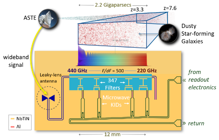 A schematic overview of the DESHIMA 2.0 chip. Image taken from [13]
DESHIMA is placed on ASTE, a ground-based sub-millimeter telescope near the ALMA site in the Atacama Desert.
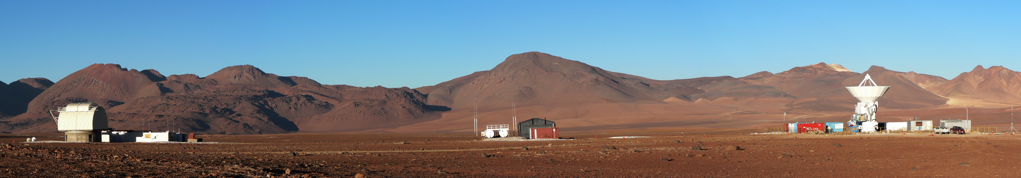 A panoramic shot from the ASTE site in the Atacama Desert. The building on the left is NANTEN-2 whereas the building on the left is ASTE. Image taken from [14]
Ground-based submillimeter astronomy
While the ASTE site is high up in the Atacama desert, the telescope still needs to look through some atmosphere when doing observations. Since cosmological object of interest are often far away and therefore very dim, they are much dimmer than the effects from the atmosphere. The atmosphere is almost completely opaque at some frequencies DESHIMA operates in and this loads the antenna dish because it is much hotter and therefore brighter than the astronomical source.
Below the atmospheric loading at the ASTE site is calculated by the software package deshima-sensitivity[15] and plotted with a galaxy spectrum synthesized by galspec:
Comparing the spectral flux density of atmospheric loading to loading from an astronomical source. The former is over 3 orders of magnitude brighter. Note how the atmospheric transmission means that for some frequencies the spectrum is barely usable.
The atmosphere is over 3 orders of magnitude brighter than the galaxy spectrum before the latter is attenuated. After the atmospheric attenuation the difference is even bigger. Therefore modeling the expected loading from the atmosphere and the entire chain from antenna to detector is important to be able to do measurements and to find the signal within the noise. deshima-sensitivity[15] was designed to do this, but takes some approximations that were deemed too reductive.
This Project
The current version of deshima-sensitivity does not take filter profiles into consideration when calculating the power received on each channel. It samples the power spectral density calculated to be at the filter's center frequency and multiplies this with the filter bandwidth, creating a crude box filter. While this approach holds for flat power spectra, it doesn't quite hold for spectra like the one above.
In this project I will modify the existing deshima-sensitivity package to more accurately resemble the DESHIMA 2.0 filter profiles and therefore the spectrometer as a whole. In order to do so, I will first need to dive into the DESHIMA system in more depth and then give an overview of photon statistics and the associated photon noise. Finally I will model the system and compare it with previous versions of deshima-sensitivity.
Bibliography
- [1]A. Einstein, “Zur Elektrodynamik bewegter Körper,” Annalen der Physik, vol. 322, no. 10, pp. 891–921, 1905, doi: 10.1002/andp.19053221004.
- [2]V. M. Slipher, “Radial velocity observations of spiral nebulae,” The Observatory, vol. 40, pp. 304–306, 1917, doi: 10.1002/andp.19053221004.
- [3]A. Lemke, “The visible light spectrum,” Once Inc. Aug-2020 [Online]. Available at: https://www.once.lighting/visible-light-spectrum/
- [4]A. Blain, “Submillimeter galaxies,” Physics Reports, vol. 369, no. 2, pp. 111–176, Jan. 2002, doi: 10.1016/s0370-1573(02)00134-5.
- [5]R. Garner, “Messier 16 (The Eagle Nebula),” NASA. NASA, Oct-2017 [Online]. Available at: https://www.nasa.gov/feature/goddard/2017/messier-16-the-eagle-nebula
- [6]A. Endo, “Session 2 | Line Emission and Cosmological Redshift ,” EE3350TU Introduction to Radio Astronomy. Nov-2020.
- [8]T. Bakx and S. Brackenhoff, “galspec v0.2.6,” pypi.org. Open Source, Nov-2020 [Online]. Available at: https://pypi.org/project/opensimplex/
- [9]A. J. Baker, From z-machines to ALMA: (sub)millimeter spectroscopy of galaxies: proceedings of a workshop held at the North American ALMA Science Center of the National Radio Astronomy Observatory in Charlottesville, Virginia, United States, 12-14 January 2006. Astronomical Soc. of the Pacific, 2007, p. 375.
- [10]E. Optics, “Introduction to Optical Prisms,” Edmund Optics. [Online]. Available at: https://www.edmundoptics.eu/knowledge-center/application-notes/optics/introduction-to-optical-prisms/
- [11]A. Endo et al., “First light demonstration of the integrated superconducting spectrometer,” Nature Astronomy, vol. 3, no. 11, pp. 989–996, 2019, doi: 10.1038/s41550-019-0850-8.
- [12]A. Endo et al., “Wideband on-chip terahertz spectrometer based on a superconducting filterbank,” Journal of Astronomical Telescopes, Instruments, and Systems, vol. 5, no. 03, p. 1, 2019, doi: 10.1117/1.jatis.5.3.035004.
- [13]E. et al. Huijten, “TiEMPO: Open-source time-dependent end-to-end model for simulating ground-based submillimeter astronomical observations,” Millimeter, Submillimeter, and Far-Infrared Detectors and Instrumentation for Astronomy X, 2020, doi: 10.1117/12.2561014.
- [14]D. R. Jacobsen, “Atacama Submillimeter Telescope Experiment complex, Chile.” English Wikipedia, 06-Jul-2008 [Online]. Available at: https://commons.wikimedia.org/w/index.php?curid=60009729
- [15]A. Endo and A. Taniguchi, “deshima-sensitivity v0.3.0,” pypi.org. Open Source, Jun-2021 [Online]. Available at: https://pypi.org/project/deshima-sensitivity/