The Model
Designing the model
- Filter distribution
- Non-flat Power Spectrum Densities
- Noise Equivalent Power
- The Filter Matrix
- Transforming the calculated noise
- The Final Model
- Bibliography
The original deshima-sensitivity code follows the following flowchart
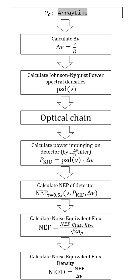 A flowchart showing the design of the old version of the model.
The optical chain described in the flowchart consists of serial transmission calculations from 1 medium to another. This entire chain of stacked transformations of the spectral input power can be regarded as a single affine transformation of the input and is independent of the bandwith or amount of frequency bins. It will remain unchanged throughout the proposed modifications.
The power impinging on a detector for a specific filter bin is calculated by taking the spectral flux density at the center frequency $\nu_c$ and multiplying this with the bandwith $\Delta\nu$. This matches the model of the previous described box filter, assuming the flux density $\mathrm{psd}$ is flat over the entire bandwith. This is not the case however, as we shall see.
Filter distribution
1 filter channel has so far been approximated as a perfect box integral, which is physically inaccurate. As we have seen, the actual filter shapes are more closely described by a Lorentzian curve
$$\begin{equation} \eta\left(\nu\right)=\frac{A\gamma^2}{\left(\nu-\nu_0\right)^2+\gamma^2} \end{equation}$$Where $\gamma$ is the half-width at half maximum (HWHM) value, for DESHIMA given as $$\begin{equation} \gamma=\frac{\nu_c}{2R} \end{equation}$$ with $R=500$ the spectral resolution. As we have seen previously our box filters were defined by an efficiency constant labeled $\eta_0$. Together with the bandwidth, this describes the transmission of the box filter. If we define the full width at half maximum for the Lorentzian as the bandwidth of the Lorentzian, we would like to define the $A$ parameter such that the area of this $\mathrm{FWHM}$ is exactly the same as the area of the box filter.
$$\begin{equation} \eta_02\gamma = \int_{\nu_0-\gamma}^{\nu_0+\gamma}\frac{A\gamma^2}{\left(\nu-\nu_0\right)^2+\gamma^2}d\nu=\frac{\pi}{2}\gamma A\Leftrightarrow A = \frac{4}{\pi}\eta_0 \end{equation}$$Meaning our filters are given by
$$\begin{equation} \eta\left(\nu\right)=\frac{4}{\pi}\frac{\eta_0\gamma^2}{\left(\nu-\nu_0\right)^2+\gamma^2} \end{equation}$$For atmospheric loading, which as you might recall is the main source of the noise, the channel is of course loaded over the entire filter spectrum: both in and out band. For a constant $\mathrm{PSD}$ this means that the corresponding box approximation can simply be widened so as to enclose the same area as the full band of the filter. For a Lorentzian this is as simple as widening the effective bandwidth with a constant:
$$\begin{equation} \int_{-\infty}^{\infty}\frac{A\gamma^2}{\left(\nu-\nu_0\right)^2+\gamma^2}d\nu=\pi\gamma A=2\int_{\nu_0-\gamma}^{\nu_0+\gamma}\frac{A\gamma^2}{\left(\nu-\nu_0\right)^2+\gamma^2}d\nu \end{equation}$$Meaning that the full band effective bandwidth is exactly twice the in band effective bandwidth.
The different sections of the Lorentzian filter. The box approximation and the corresponding part of the Lorentzian have the same area.
Noise Equivalent Power
Redoing the calculation of the noise equivalent power for a flat $\mathrm{PSD}$, but with proper Lorentzian filters $\eta\left(\nu\right)$ this time, results in:
$$\begin{equation} \begin{split} \mathrm{NEP}_{\tau=0.5\mathrm{s},\mathrm{ph}}^2&=2\int_0^\infty h\nu\eta(\nu)\mathrm{PSD}+\eta^2(\nu)\mathrm{PSD}^2d\nu\\ &=2\mathrm{PSD}\int_0^\infty h\nu\eta(\nu)d\nu+2\mathrm{PSD}^2\int_0^\infty \eta^2(\nu)d\nu \\ &\approx8\mathrm{PSD}h\nu_0\eta_0\gamma + \frac{16}{\pi}\mathrm{PSD}^2\eta_0^2\gamma \\ &=4\mathrm{PSD}h\nu_0\eta_0\mathrm{FWHM}+\frac{8}{\pi}\mathrm{PSD}^2\eta_0^2\mathrm{FWHM} \end{split} \end{equation}$$where an approximation is used for the first term, assuming $\Delta\nu\ll\nu$. Because the calculations are done for a constant $\mathrm{PSD}$, the filter gets loaded across the full band, meaning the effective bandwidth $\Delta\nu=2\mathrm{FWHM}$. Putting this in the equation for the $\mathrm{NEP}_{\tau=0.5\mathrm{s},\mathrm{ph}}$ yields:
$$\begin{equation} \begin{split} \mathrm{NEP}_{\tau=0.5\mathrm{s},\mathrm{ph}} &= 2\mathrm{PSD}\eta_0\Delta\nu h\nu_0+\frac{4}{\pi}\mathrm{PSD}^2\eta_0^2\Delta\nu \\ &=2P_\mathrm{KID}h\nu_0 + \frac{4}{\pi}\frac{P^2_\mathrm{KID}}{\Delta\nu} \end{split} \end{equation}$$Which means the second term, the bunching term, is a factor of $\pi/2$ smaller than is the case for narrow-bandwidth approximation described in [1] and used in [2]. This can be explained because the full Lorentzian has a non-negligible width and therefore the approximation of $\nu\gg\Delta\nu$ from [1] doesn't hold. In other words the photons impinging on the detector span a bigger bandwidth than previously approximated and therefore bunch less.
Non-flat Power Spectrum Densities
We know the $\mathrm{NEP}$ is proportional to the $\mathrm{PSD}$ impinging on the detector, and we have also seen that the atmospheric loading is a much bigger contribution to the spectral flux density than any astronomical source. Let's take a look at how this atmospheric loading varies over the bin width. In the figures below the actual target frequency channels from DESHIMA 2.0 are taken and compared to the atmospheric model measured at ASTE, taken from deshima-sensitivity.
A non-flat power spectral density overlayed over box filters. The out of band loading is not calculated.
For the channels where the atmospheric loading is reasonably constant over the bandwidth this approximation is fine, however when the spectral flux density peaks to twice it's local background level the box filters are obviously a poor approximation for reality. The atmospheric loading is averaged over the bandwidth before being multiplied with it in the current version of deshima-sensitivity, in essence integrating it over the box filter. However, this crude approximation clearly fails when looking at the actual Lorentzian filters.
A non flat power spectral density overlayed over Lorentzian filters. Here filters are loaded out of band.
The peak at $286.1\:\mathrm{GHz}$ is obviously loading channel 131 and 132, but due to the wide profile of a Lorentzian even 130 and 133 are receiving energy from the peak in flux density.
The total power impinged on the detector can be approximated by calculating the spectral power arriving at the detector not just at the center frequencies of the bins $\nu_0$, but by expanding the number of frequencies calculated to some amount of integration bins and calculating the spectral power at these frequencies. For an integration frequency $\nu_i$ and a channel $j$, the effective power loading by that frequency on that channel is given by:
$$\begin{equation} P_{\mathrm{KID},i,j} = \eta\left(\nu_i,j\right)\mathrm{PSD}\left(\nu_i\right)\Delta\nu_i\label{p_kid_i} \end{equation}$$with $\Delta\nu_i$ the bandwidth for that frequency. The total power impinged on a filter channel $P_{\mathrm{KID},j}$ is then given by:
$$\begin{equation} P_{\mathrm{KID},j}=\sum_i P_{\mathrm{KID},i,j} = \sum_i \eta\left(\nu_i,j\right)\mathrm{PSD}\left(\nu_i\right)\Delta\nu_i \label{p_kid} \end{equation}$$To make this more visual, take a look at the figure below
A stem plot of the power spectral density overlayed over binned Lorentzian filters.
The calculated flux spectrum arriving at the filter will be calculated as is done in the current version of the deshima-sensitivity package, but using a finer frequency resolution. This spectrum will then arrive at the filter, where for each channel a weighted sum will be taken over all integration bins, resulting in a total power impinged on the detector.
Noise Equivalent Power
As seen, the photon noise equivalent power for a single DESHIMA channel $\mathrm{NEP}_{\tau=0.5\mathrm{s},\mathrm{ph},j}$is given by[1]:
$$\begin{equation} \mathrm{NEP}_{\tau=0.5\mathrm{s},\mathrm{ph},j}^2=2\int_0^\infty h\nu\eta\left(\nu,j\right)\mathrm{PSD}\left(\nu\right)+\eta^2\left(\nu,j\right)\mathrm{PSD}\left(\nu\right)^2d\nu \end{equation}$$Again taking the filter efficiency $\eta\left(\nu_i,j\right)$ and $\mathrm{PSD}$ constant over a single integration frequency, and multiplying $\mathrm{PSD}$ with the bandwidth to get the power impinged by an integration bin on the channel $P_{\mathrm{KID},i}$ we can easily take the Riemann sum of this integral as
$$\begin{equation} \mathrm{NEP}_{\tau=0.5\mathrm{s},\mathrm{ph},j}^2=2\sum_i\left( h\nu_iP_{\mathrm{KID},j,i}+\frac{P_{\mathrm{KID},j,i}^2}{\Delta\nu_i}\right)\label{nep_ph} \end{equation}$$The recombination noise $\mathrm{NEP_{R}}$ is given by
$$\begin{equation} \mathrm{NEP}_{\tau,\mathrm{R},j}^2=\frac{1}{\tau}2\Delta_\mathrm{Al}\frac{P_{\mathrm{KID},j}}{\eta_\mathrm{pb}}=\frac{1}{\tau}2\Delta_\mathrm{Al}\frac{\sum_i{P_{\mathrm{KID},j,i}}}{\eta_\mathrm{pb}} \end{equation}$$Which results in a total $\mathrm{NEP}_{\tau=0.5\mathrm{s}}$ of
$$\begin{equation} \mathrm{NEP}_{\tau=0.5\mathrm{s},j} = \sqrt{2\sum_i\left( h\nu_iP_{\mathrm{KID},j,i}+\frac{P_{\mathrm{KID},j,i}^2}{\Delta\nu_i}\right) + 4\Delta_\mathrm{Al}\frac{\sum_i{P_{\mathrm{KID},j,i}}}{\eta_\mathrm{pb}}}\label{total_NEP} \end{equation}$$Photon Bunching
But what about photon bunching? I have shown that the coherence time and the bandwidth are inversely proportional. By decreasing the size of the integration bins we have also decreased the bandwidth and therefore increased the coherence time.
Now the $\mathrm{NEP}$ is simply defined at $\tau=0.5\:\mathrm{s}$, but in measurements the integration time can vary. The $\mathrm{NEP}$ is scaled accordingly:
$$\begin{equation} \begin{split} \mathrm{NEP}_{\tau,j} &= \frac{1}{\sqrt{\tau}}\sqrt{\sum_i\left( h\nu_iP_{\mathrm{KID},j,i}+\frac{P_{\mathrm{KID},j,i}^2}{\Delta\nu_i}\right) + 2\Delta_\mathrm{Al}\frac{\sum_i{P_{\mathrm{KID},j,i}}}{\eta_\mathrm{pb}}} \\ &=\frac{1}{\sqrt{2\tau}}\mathrm{NEP}_{\tau=0.5\mathrm{s},j} \end{split} \end{equation}$$Even though DESHIMA 2.0 samples at a minimum integration frequency of $160\:\mathrm{Hz}$ which results in a integration time of $\tau=6.25\:\mathrm{ms}$, it still integrates periods orders of magnitude longer than the coherence time [3], meaning that the non-stochastic effects of photon bunching still don't come into play and we can define the noise as described previosuly.
But this scaling doesn't hold indefinitely. I conjecture that at some point the incoming photons are sampled at such a short sampling interval that they become correlated, as we have seen previously. In order to investigate this, let's define 3 bunched signal using open simplex noise[4] as done before along with an uncorrelated signal, where the underlying probability doesn't change, as in the first example of the previous section.
The autocorrelation of three different bunched signals, with coherence times at roughly 10, 20 and 50 steps along with a totally uncorrelated signal.
Here the signals are generated such that they have a coherence time $t_\mathrm{coh}$ of roughly 10, 20 and 50 steps. By sampling these signals at sampling intervals much longer than the coherence time $t_\mathrm{sample}\gg t_\mathrm{coh}$ we get the same inverse square root relation as we have derived for the $\mathrm{NEP}_{\tau}$. However when the sampling time nears the coherence time this relation no longer holds. Since detections shorter than a coherence time apart are correlated the overall uncertainty drops.
When the sampling time drops below the coherence time the inverse square root relation doesn't hold any longer.
This result shows the difference between the stochastic and the non-stochastic effects of photon bunching. It is the reason why we can model the bunching term as white noise as long as the integration time $\tau$ stays clear of the coherence time.
The Filter Matrix
From eq \eqref{p_kid_i} we can see that we need a two dimensional function $\eta\left(\nu_i,j\right)$ to go from a one dimensional $\mathrm{PSD}$ to a power spectrum for each filter channel. We do this programmatically by calculating a matrix that takes in a vector containing the $\mathrm{PSD}$ at each integration frequency and use that to calculate the power loading by this $\mathrm{PSD}$ on each channel.
Shown in the figure below is a visualization of how this filter matrix might look like.
A visual interpretation of the filter matrix. Only 20 channels are shown.
With this framework in place it is easy to swap out the generated filter with another, more realistic model of the filters. The figure below shows a simulated filter transmission curve for the DESHIMA 2.0 chip.
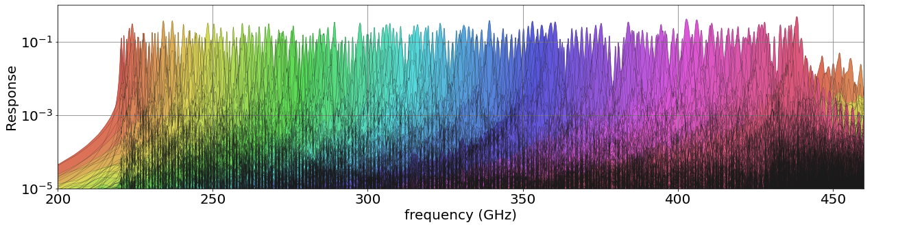 A simulated filter profile of the DESHIMA 2.0 spectrometer
As you can see, the filters aren't all equally efficient and wide, nor are they perfectly Lorentzian. In the figure below all 346 bins and the corresponding values of $R$ are plotted, with the size corresponding to the transmission.
The variations of this simulated filter are clear in this plot. The size corresponds to the transmission. Hover over and the χ2 parameter of the fit is shown for each channel.
While using a perfect Lorentzian approximation for the filter profiles for each channel is better than the center frequency sampling that is done now, it might be more advantageous to be able to use simulated or measured profiles. The filter matrix will therefore, depending on the users choice, be either generated via Lorentzian curves or loaded in via a file.
Transforming the calculated noise
Once the $\mathrm{NEP}$ has been calculated, it needs to be compared to a source in order to calculate the signal to noise. This can be done by generating various signals that are fed through the entire optical chain again and compare the power these impart on the detectors to the $\mathrm{NEP}$ we calculated. Another, crude but nevertheless convenient estimation can be acquired by transforming the noise back into more usable and define the sensitivity of the instrument that way. This model will focus on the latter.
We calculate the source coupling through a quantity named the Noise Equivalent (Source) Flux $\mathrm{NEF}$. The $\mathrm{NEF}$ is defined as the flux a source needs to impinge on the detector for it to equal the $\mathrm{NEP}$ in strength and is therefore our sensitivity: a source with a flux lower than the $\mathrm{NEF}$ will be hidden in the noise of the measurement data during an integration time of $1\:s$. Take note that the $\mathrm{NEF}$ is defined for an integration time of $\tau=1\:\mathrm{s}$, rather than $\tau=0.5\:\mathrm{s}$ as is the case for the $\mathrm{NEP}$. The $\mathrm{NEF}$ is given by: $$\begin{equation} \mathrm{NEF} =\frac{\mathrm{NEP_{inst,{\tau=0.5\mathrm{s}}}}}{\eta_\mathrm{sw}\sqrt{2}A_g}=\frac{\mathrm{NEP}_{\tau=0.5\mathrm{s}}}{\eta_\mathrm{inst}\eta_\mathrm{sw}\sqrt{2}A_g} \end{equation}$$
with $A_g$ the area of the telescope, $\eta_\mathrm{sw}$ the aggregate efficiency from the source up to and including the window of the cryostat chamber DESHIMA is housed in and $\eta_\mathrm{inst}$ the instrument efficiency: the aggregate of all the efficiencies within the cryostat. The first two remain unchanged throughout the modifications discussed in this chapter, however $\eta_\mathrm{inst}$ is dependent on the filter efficiency and is therefore modified.
Since the calculation of the $\mathrm{NEP}_{\tau=0.5\mathrm{s}}$ as in \eqref{total_NEP} collapses the noise equivalent power down to a single value per channel, we can't use the efficiency as calculated for the integration bins to go back through the system in order to calculate the source coupling. Instead there are two different approximations we can take to calculate the source coupling: an in-band and a full band approximation
In-band Source Coupling
The in-band approximation is used for spectral sources. A spectral source is defined as an object that transmits only within the bandwidth of a single filter channel, where we define the bandwidth as the $\mathrm{FWHM}$
A spectral source is defined as a source that fully fits within the bandwidth of a channel. Shown here for a Lorentzian filter
In order to get a single value of an efficiency, let's say $\eta_\mathrm{inst}$, over the full in-band bandwidth, I take a weighted average over the $\mathrm{FWHM}$ where the weights are given by the filter efficiency $\eta\left(\nu,j\right)$.
$$\begin{equation} \eta_\mathrm{inst,j}=\frac{\int_{\nu_j-\gamma}^{\nu_j+\gamma}\eta_\mathrm{inst}\left(\nu\right)\eta\left(\nu,j\right)d\nu}{\int_{\nu_j-\gamma}^{\nu_j+\gamma}\eta\left(\nu,j\right)d\nu} \end{equation}$$This ensures that the efficiency per channel is normalized such that I can use the box-filter approximation on our way back through the system.
Because spectral sources fit within the bandwidth of a single channel, the box-approximation holds very well.
The continuum of blackbody radiation loads the entire channel. Because it varies so slowly over the channel, it can be assumed as constant over a channel and the box filter approximation holds too.
Because this continuum source is as near as makes no difference constant over the frequency bin, we can model it's transmission by another box-filter, with double the bandwidth of the spectral case, as I have derived previously.
In this case, the efficiencies are calculated using another weighted average, weighted over the full band this time
$$\begin{equation} \eta_\mathrm{inst,j}=\frac{\int_0^\infty\eta\left(\nu\right)\eta\left(\nu,j\right)d\nu}{\int_0^\infty\eta_\mathrm{filter}\left(\nu,j\right)d\nu} \end{equation}$$The Final Model
Using these two approximations, the NEP can be transformed back through the system and to the sky again as the $\mathrm{NEF}$. In order to transform the $\mathrm{NEF}$ to a flux density, we simply divide by the effective bandwidth for either the line or spectral case and get the noise equivalent flux density $\mathrm{NEFD}$.
This means that the total model looks like this:
 The updated model. Noteworthy changes are the filter and the parallel line and spectral source paths.
Bibliography
- [1]J. Zmuidzinas, “Thermal noise and correlations in photon detection,” Applied Optics, vol. 42, no. 25, p. 4989, 2003, doi: 10.1364/ao.42.004989.
- [2]A. Endo et al., “First light demonstration of the integrated superconducting spectrometer,” Nature Astronomy, vol. 3, no. 11, pp. 989–996, 2019, doi: 10.1038/s41550-019-0850-8.
- [3]B. L. Morgan and L. Mandel, “Measurement of Photon Bunching in a Thermal Light Beam,” Physical Review Letters, vol. 16, no. 22, pp. 1012–1015, 1966, doi: 10.1103/physrevlett.16.1012.
- [4]K. Spencer and O. S. Community, “opensimplex v0.3,” pypi.org. Open Source, Dec-2021 [Online]. Available at: https://pypi.org/project/opensimplex/