Photon Statistics
Photon Statistics and the unintuitive way photons behave when they arrive sparsely
Because of the inherent probability quantum mechanics entails, photons arriving at some detector follow statistical properties. In this chapter I will discuss these Photon Statistics and the unintuitive way photons behave when they arrive sparsely.
Photon Noise
In order to quantify the sensitivity of a DESHIMA type spectrometer, we need to know the amount of noise that is generated by the aforementioned atmospheric and optical loading and compare this to the signal that an observation will impart on the detector. For our purposes this noise consists of photon noise and quasiparticle recombination noise, the first of which can be split up into two categories: thermal noise and shot noise.
An observed astronomical object also emits random photons that reach the detector, therefore contributing to photon noise[1]. While this won't be included in the model, as the model is designed such that it calculates the noise when off-source, the following topics in this chapter are equally valid for photon noise emitted and caused by the astronomical source.
Thermal Noise
In radio receivers, a big part of the noise is generated by thermal agitation of electrons. In most uses this can be classified as white noise:the power is constant across its frequency spectrum [2], but in extremely high frequencies or low temperatures this approximation doesn't hold. The power $P$ transmitted by the noise is given as Johnson-Nyquist Noise and is approximated for small bandwidths $\Delta\nu$ as[3]: $$\begin{equation} P=\int_{\nu_0}^{\nu_1}\frac{h\nu}{e^{h\nu/k_BT}-1}d\nu \approx \frac{h\nu}{e^{h\nu/k_BT}-1}\Delta\nu = P_\nu\Delta\nu \end{equation}$$
With $P_\nu$ the power spectrum in $\mathrm{[WHz^{-1}]}$. Plotting the normalized ($P_\nu/k_BT$) power spectrum supports my earlier statements that, in most cases, thermal noise can be approximated as white
Comparing the normalized Johnson-Nyquist noise for different temperatures shows that it is white for low frequencies
Unfortunately, this white noise approximation starts to break down in atmospheric temperature for the DESHIMA range. Once more, it is also not the only form of noise we have to deal with.
Shot noise
When the source is very dim, photons arrive one at a time. This means that we are dealing with shot noise[1]. Here the detection rate of a photon is characterized by Poisson statistics and the famous Poisson distribution [4]:
$$\begin{equation} f(x)=\frac{\lambda^xe^{-\lambda}}{x!} \end{equation}$$Hence we also call this noise Poisson noise.
Typical Poisson curves for different parameters.
Uncertainty
From Poisson statistics we know that the uncertainty $\sigma_N$ over some number of counts or occurrences $N$ is equal to the square root of the number of counts, since it's an uncorrelated process [1][4]. Because our power arrives with single photons hitting the detector, the power follows the same uncertainty
$$\begin{equation} \sigma_N=\sqrt{N} \end{equation}$$$$\begin{equation} \sigma_P \propto \sqrt{P} \end{equation}$$However, if we look at Johnson-Nyquist noise and approximate for lower frequencies we get[1][3]:
$$\begin{equation} P \approx \frac{h\nu}{e^{h\nu/k_BT}-1}\Delta\nu \approx k_BT\Delta\nu \end{equation}$$$$\begin{equation} \sigma_P \propto P \end{equation}$$Hence we have found two proportionality relations for the uncertainty, which is it?
Particle-Wave duality
The seemingly paradoxical nature of this uncertainty can be explained as a caveat of the particle-wave duality. In the wave domain the Johnson-Nyquist noise dominates, whereas in the particle domain we get mainly Poisson noise. The general case of the uncertainty in the rate of photons arriving within a detection time of $\tau$ is[5][6]:
$$\begin{equation} \sigma_\mathrm{ph}= \frac{1}{\sqrt{\tau}}\sqrt{n^2+n}\label{simple_sigma_ph} \end{equation}$$with $n$, the photon number, being the number of photons arriving per time per bandwidth. Here both extremes are more obvious: for $n\gg 1$ we get the thermal noise from the wave domain and for $n \ll 1$ the Poisson uncertainty falls out.
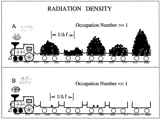 An analogy for the detection of photons in the particle and wave limit. Image taken from [1]
The photon number for a thermal blackbody radiator is given by the Bose-Einstein equation [7][6]
$$\begin{equation} n_\mathrm{th}\left(\nu,T\right)=\frac{1}{e^{h\nu/k_BT}-1} \end{equation}$$Which means that in the region between $220\:{\mathrm{GHz}}$ and $440\:{\mathrm{GHz}}$ the photon occupation number is neither fully in the wave limit nor the particle limit.
The photon number for different temperatures is neither fully in the wave limit nor fully in the particle limit in the DESHIMA range
In the wave domain, where the photon number is higher, photons tend to come clumped together in a process known as photon bunching[6], which explains the increase in noise.
Photon Bunching
Quantum Electrodynamics has taught us that photons behave stochastically, so it is reasonable to assume that photon detection also occurs randomly. While this is (obviously) true to some degree, in the previous section I stated photons can arrive 'clumped' together at the detector in a phenomenon known as photon bunching. This means that detecting one photon will result in a higher chance of another photon being detected within a specified time, called the coherence time $t_{\mathrm{coh}}$ [6]. In this chapter I will first present an intuitive, qualitative explanation as to why photon bunching occurs. Then I will go deeper into the mathematics and quantum mechanics of photon bunching and the specific case of the DESHIMA system.
An analogy
To understand photon bunching, first think of photons arriving at the detector like raindrops falling on a piece of paper. While it's raining with constant intensity, the chance of a raindrop falling on a specific area within, say, the next second (expressed by $P(\mathrm{drop})$) is constant. In the figure below I have set $P(\mathrm{drop}) = 0.3$:
Plotting occurrences and the underlying probability for a constant chance.
The raindrops fall uncorrelated: every second a new chance of $P(\mathrm{drop})$ means a raindrop falling from the sky might land in our defined area. This is how unbunched, or random, photons behave.
Now let's assume the chance of a raindrop occurring is not constant over time, but rather varies relatively slowly over time. This could be because of varying wind speeds or varying intensity in the rain, but whatever the case the rain drops are no longer uncorrelated. There are moments of high intensity, where the chance of a raindrop is high and similarly there are moments of low intensity. I have simulated this using open simplex noise [8] in the following graph.
Plotting occurrences and the underlying probability for a varying chance.
As is clear from the graph, the raindrops are clumped together. This is the same underlying principle as photon bunching in photons from astronomical sources. The random motion of the exciting atoms, for example Brownian motion, means that the intensity also fluctuates over time[6]. It is therefore not the act of detecting a photon that increases the chance of another detection, but rather an underlying change in probability of detecting, easily explained by probabilistics.
This means that at the point where a raindrop falls or a photon gets emitted, it is still a simple stochastic process. Should our sampling interval be much smaller than the time over which the rain varies, we'd still see 'stochastic regions', where the probability function stays roughly constant, like in the first example. This is illustrated in the graph below with stretched noise:
Plotting occurrences and the underlying probability for a slowly varying chance.
The droplets appear less bunched, because the time scale in which the measurements take place is much smaller than the time scale in which the intensity changes. The very first example I spoke about, of raindrops falling at a constant intensity, is a situation in which this discrepancy occurs. Of course it won't rain forever and when the rain dies down the chance of a raindrop falling is much lower than while it's still raining. So while the droplets look purely random when it rains, they aren't over the course of the entire day. I will call this behavior bunched (slow timescale), because the sampling time is much faster than the coherence time, which I shall later elaborate on further.
Let's also take a look at what happens when the sampling time is much slower than the underlying probability fluctuations.
Plotting occurrences and the underlying probability for a quickly varying chance.
As expected, the detection rate looks much like the first detection rate with constant $P\left(\mathrm{drop}\right)$. Although the underlying probability changes, it changes too fast between detections for bunching to occur.
Intermezzo: Antibunching
While this report focuses on photon bunching, the opposite also occurs in, for example, single photon sources [9]. Now that I have discussed a framework with which to explain photon bunching, I thought it would be remiss to leave out an explanation for antibunching.
As one would expect, in antibunching the opposite of bunching happens: detecting a raindrop would mean that, at least for the next period of time, the chance of a raindrop falling becomes smaller. A good allegory for this is a dripping faucet. A small flow of water exits the faucet and, due to surface tension, pools up in a small droplet at the end. As the droplet gets bigger, the chance of it falling increases, but once it drips down it takes all water with it and the process starts anew.
An analogy for anti-bunching.
This behavior corresponds with antibunching behavior in single photon sources[9]. Atoms are excited through an energy pump process. When this energy increases sufficiently they emit a photon and lose energy, ready to get excited again[6].
Again, the detection of such single photons will display antibunching, but it is not the detection that triggers this cool-down period, it is the emission.
All different probability and occurrences for the discussed probabilities. These are toggleable By selecting modes in the legend.
Coherence
If the underlying probability function is unknown (and quantum mechanically it is), how would we be able to quantify whether our detections are bunched. A possible heuristic we can use comes from signal processing. We could take the autocorrelation of the signals and compare them. Since the autocorrelation is the cross-correlation between the signal and a time-shifted copy, we'd likely see the bunched signal display some sort of correlation for a delay that is around the timescale of the oscillations in the probability function. In the figure below I have correlated the detections described above with $t\in[0,10000]$ and plotted these values for different time delays $h$.
The autocorrelation for the different photon modes.
As is clear from the graph, the bunched photons show some autocorrelation, with the longer timescale showing longer (bigger time shifts) autocorrelation. This can be explained further by signal analysis. We are working in the discrete domain and smaller sampling steps relative to the variation in the underlying probability will mean more correlation.
What this shows is temporal coherence, a property of light that describes the predictability over a timescale[1].
Bandwidth
Up until now we have only looked at raindrops as analogous detections, but when talking about photons we need to take frequency into account. Photons obey the Heisenberg uncertainty relation where the uncertainty in position $\Delta x$ and momentum $\Delta p_x$ must obey [1]:
$$\begin{equation} \Delta x\Delta p_x = \frac{\hbar}{2} \end{equation}$$Our photons are flying at the detector, so its uncertainty in longitudinal ($z$, towards the detector) position can be equated as it's uncertainty in detection time and it's momentum can be expressed as $h/\lambda$:
$$\begin{equation} \Delta z \cdot\Delta p_z= c\Delta t\cdot\frac{h\Delta\nu}{c} = h\Delta t\Delta\nu = \frac{\hbar}{2} \end{equation}$$and finally we arrive at
$$\begin{equation} \Delta\nu \propto \frac{1}{\Delta t} \end{equation}$$In other words: a shorter coherence time means more accurate knowledge on where the photons are, meaning their uncertainty in momentum and therefore bandwidth is bigger.
This relation can also be seen experimentally. In Morgan and Mandel's 1966 paper[10], the authors explore the autocorrelation between two different light sources: a Hg198 source with a very narrow bandwidth (a) and a tungsten light bulb with a broad spectrum thermal source (b). By designing an apparatus that counts the number of times two photon arrive within a defined time period, they show the autocorrelation of the two light sources
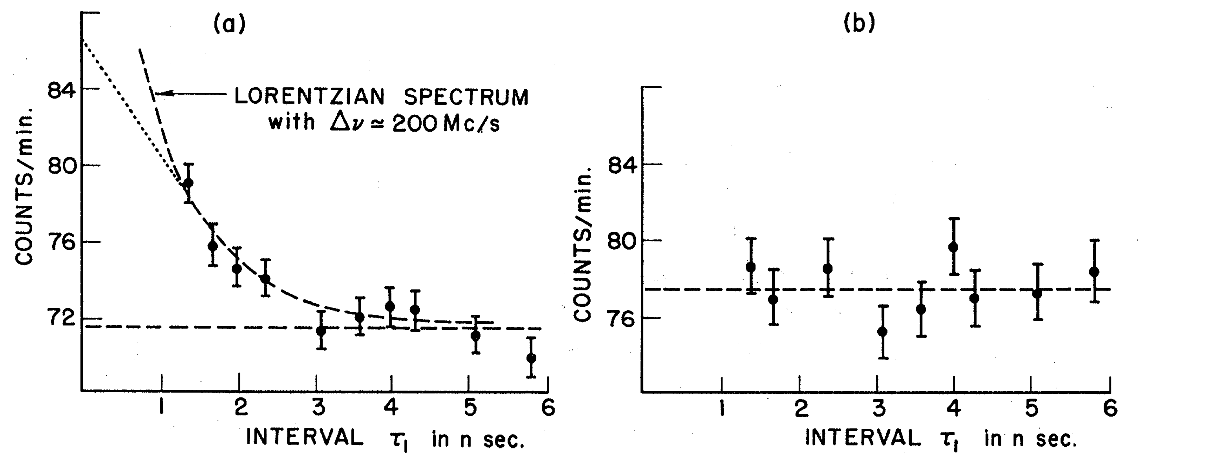 The number of times per second two photons arrived after a specified time delay for a a) Hg198 light source and a b) tungsten incandescent light source. Image taken from [10]
Because the tungsten light has a wide bandwidth, it has a short coherence time and the reverse is true for the Hg198 light. Therefore, if we take the short timescale bunched photons as an analogy for the tungsten light and the longer timescale bunched lights as analogous for the mercury light, we get something that looks very similar.
The autocorrelation of just the slow and short bunched timescale photons behave like the spectral and tungsten source respectively.
With a more thorough understanding of photon bunching, it is time to return to photon noise and discuss noise-equivalent power.
Noise Equivalent power
The noise equivalent power ($\mathrm{NEP}$) is a way to express the sensitivity of a photon detector. It is defined as the input signal power that results in a signal-to-noise-ratio of 1 in a 1 Hz output bandwidth. [11]. For our purposes this means multiplying the uncertainty in photon count $\sigma_\mathrm{ph}$ with the photon energy[12] and setting the $\tau$ in eq. \eqref{simple_sigma_ph} to $\tau=0.5\:\mathrm{s}$. From [7] we have an equation for the electrical (detected) photon noise
$$\begin{equation} \sigma_\mathrm{ph}^2=\frac{1}{\tau}\int_0^\infty\eta(\nu)n(\nu)\left[1+\eta(\nu)n(\nu)\right]d\nu \end{equation}$$Where $\eta\left(\nu\right)$ is the quantum efficiency, which for our purposes is the efficiency of the filter. Multiplying this integral with the photon energy, we get the electrical Noise Equivalent Power added by photon noise for a specified integration time
$$\begin{equation} \mathrm{NEP}_{\tau,\mathrm{ph}}^2=\frac{1}{\tau}\int_0^\infty\left(h\nu\right)^2\eta(\nu)n(\nu)\left[1+\eta(\nu)n(\nu)\right]d\nu \end{equation}$$This integral implicitly assumes an infinite coherence time, since it integrates over infinitely small bandwidths $d\nu$. Another side effect of this is that photons only bunch with photons that share the exact same frequency. These two paradoxical conclusions make this integral therefore inherently not physical and we will need to make some assumptions in order to work with it.
If we were to create a perfect box filter, and approximate the photon number as constant over this filter $\eta\left(\nu\right)$ falls out of the integral. Let's first define this box function
$$\begin{equation} \Pi^{\Delta\nu}_{\nu_0}(\nu)= \left\{ \begin{array}{ll} 1 & |\nu-\nu_0|\le\frac{\Delta\nu}{2} \\ 0 & \mathrm{elsewhere} \\ \end{array} \right. \end{equation}$$And then set $\eta(\nu)=\eta_0\Pi^{\Delta\nu}_{\nu_0}(\nu)$. When we assume we have a constant photon occupation number over this range, the equation simplifies to:$$\begin{equation}\begin{split} \mathrm{NEP}_{\tau,\mathrm{ph}}^2&=\frac{1}{\tau}\int_0^\infty\left(h\nu\right)^2\eta_0\Pi^{\Delta\nu}_{\nu_0}(\nu)n(\nu)\left[1+\eta_0\Pi^{\Delta\nu}_{\nu_0}(\nu)n(\nu)\right]d\nu \\ &= \frac{1}{\tau}\int_{\nu_0-\frac{\Delta\nu}{2}}^{\nu_0+\frac{\Delta\nu}{2}}\left(h\nu\right)^2\eta_0n\left[1+\eta_0n\right]d\nu \end{split} \end{equation}$$
Which, for $\Delta\nu\ll\nu$ approximates as: $$\begin{equation} \mathrm{NEP}_{\tau,\mathrm{ph}}^2=\frac{1}{\tau}\left(h\nu_0\right)^2\eta_0n\left[1+\eta_0n\right]\Delta\nu \end{equation}$$
Taking our definition of Noise Equivalent Power $\tau=0.5\:\mathrm{[s]}$, this results in a Noise Equivalent Power of:
$$\begin{equation} \mathrm{NEP}_{\tau=0.5\mathrm{s},\mathrm{ph}}=h\nu_0\sqrt{2\eta_0n\left(1+\eta_0n\right)\Delta\nu} \end{equation}$$DESHIMA
In actual measurements the photon occupation number isn't known, but we are able to deduce it from the power spectral density[6]:
$$\begin{equation} n_\mathrm{ph}=\frac{\mathrm{PSD}}{h\nu} \end{equation}$$Inserting this in the equation for $\mathrm{NEP}$ we get:
$$\begin{equation} \mathrm{NEP}_{\tau=0.5\mathrm{s},\mathrm{ph}}=\sqrt{2\eta_0\mathrm{PSD}h\nu_0\left(1+\eta_0\frac{\mathrm{PSD}}{h\nu_0}\right)\Delta\nu} \end{equation}$$If we assume the $\mathrm{PSD}$ to be flat, for a box filter the power spectrum multiplied by the bandwidth and the efficiency is obviously the power on the detector.
$$\begin{equation} P_\mathrm{KID}=\eta_0\mathrm{PSD}\Delta\nu_0 \end{equation}$$rearranging we get:
$$\begin{equation} \mathrm{NEP}_{\tau=0.5\mathrm{s},\mathrm{ph}}=\sqrt{2P_\mathrm{KID}h\nu_0 + 2\frac{P^2_\mathrm{KID}}{\Delta\nu}} \end{equation}$$Which is in agreement with [13].
Generation-Recombination Noise
Besides photon noise (both Poisson and bunching), another type of noise adds to our $\mathrm{NEP}$: recombination noise. This is a type of noise that occurs in superconductor-based pair-breaking photon detectors. As mentioned before, incoming photons generate quasiparticles in the detector, which later recombine in a Cooper pair [14]. For our purposes we will take the noise equivalent power of recombination noise $\mathrm{NEP_{\tau,R}}$ as given by [13]:
$$\begin{equation} \mathrm{NEP_{\tau,R}}=\frac{1}{\sqrt{\tau}}\sqrt{2\Delta_\mathrm{Al}\frac{P_\mathrm{KID}}{\eta_\mathrm{pb}}} \end{equation}$$Even though the amount of quasiparticles generated is proportional to the incoming power, the recombination noise happens randomly and is therefore an uncorrelated process. This means we can add the $\mathrm{NEP_R}$ and $\mathrm{NEP_{ph}}$ together by quadrature addition, creating a total noise equivalent power given by:
$$\begin{equation} \mathrm{NEP}_{\tau=0.5\mathrm{s}} = \sqrt{\mathrm{NEP}_{\tau=0.5\mathrm{s},\mathrm{ph}}^2 + \mathrm{NEP_{\tau=0.5s,R}}^2} \end{equation}$$$$\begin{equation} \mathrm{NEP}_{\tau=0.5\mathrm{s}}=\sqrt{2P_\mathrm{KID}h\nu_0 + 2\frac{P_\mathrm{KID}^2}{\Delta\nu}+4\Delta_\mathrm{Al}\frac{P_\mathrm{KID}}{\eta_\mathrm{pb}}} \end{equation}$$Finally, quasiparticles also generate randomly without any incoming photons, eg when the detector is kept in total darkness[15]. This is called Generation-Recombination noise and is negligible compared to the photon noise and photon-induced recombination noise as can be seen in the figure below:
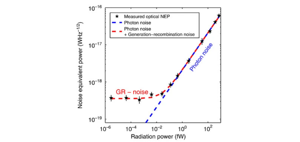 The noise induced by spontaneous Generation and recombination of quasiparticles is negligible compared to photon noise. Image taken from [15]
Because this effect is negligible, it won't be included in the model.
Bibliography
- [1]G. B. Taylor, C. L. Carilli, and R. A. Perley, Synthesis imaging in radio astronomy II: a collection of lectures from the Sixth NRAO/NMIMT Synthesis Imaging Summer School held at Socorro, New Mexico, USA, 17-23 June 1998. Astronomical Society of the Pacific, 2008, pp. 671–688.
- [2]C. S. Turner, “Johnson Nyquist noise - clay’s DSP Page,” Johnson-Nyquist Noise. Wireless Systems Engineering, Inc., Jan-2007 [Online]. Available at: http://www.claysturner.com/dsp/Johnson-Nyquist%20Noise.pdf
- [3]A. Endo, “Session 4 | Photon Noise,” EE3350TU Introduction to Radio Astronomy. Dec-2020.
- [4]F. M. Dekking, C. Kraaikamp, L. H.P, and L. E. Meester, A modern introduction to probability and statistics: Understanding why and how. Springer-Verlag, 2011.
- [5]A. Endo, “Memo: Poisson limit and bunching limit of photon NEP: Deshima Kibela,” Memo: Poisson limit and Bunching limit of Photon NEP. Kibela, Nov-2020 [Online]. Available at: https://deshima.kibe.la/shared/entries/96349e15-acfa-474f-adf8-f21ebe25cda5
- [6]H. Paul, Introduction to quantum optics: from light quanta to quantum teleportation. Cambridge University Press, 2004, pp. 127–153.
- [7]J. Zmuidzinas, “Thermal noise and correlations in photon detection,” Applied Optics, vol. 42, no. 25, p. 4989, 2003, doi: 10.1364/ao.42.004989.
- [8]K. Spencer and O. S. Community, “opensimplex v0.3,” pypi.org. Open Source, Dec-2021 [Online]. Available at: https://pypi.org/project/opensimplex/
- [9]M. Krottenmüller, “Photon Statistics,” Technische Universität München. May-2013 [Online]. Available at: https://www.mpq.mpg.de/5020834/0508a_photon_statistics.pdf
- [10]B. L. Morgan and L. Mandel, “Measurement of Photon Bunching in a Thermal Light Beam,” Physical Review Letters, vol. 16, no. 22, pp. 1012–1015, 1966, doi: 10.1103/physrevlett.16.1012.
- [11]P. L. Richards, “Bolometers for infrared and millimeter waves,” Journal of Applied Physics, vol. 76, no. 1, pp. 1–24, 1994, doi: 10.1063/1.357128.
- [12]S. Leclercq, “Discussion about Noise Equivalent Power and its use for photon noise calculation,” 2007 [Online]. Available at: https://www.iram.fr/ leclercq/Reports/About_NEP_photon_noise.pdf
- [13]A. Endo et al., “First light demonstration of the integrated superconducting spectrometer,” Nature Astronomy, vol. 3, no. 11, pp. 989–996, 2019, doi: 10.1038/s41550-019-0850-8.
- [14]P. J. de Visser, “Quasiparticle dynamics in aluminium superconducting microwave resonators,” Mar. 2014, doi: 10.4233/uuid:eae4c9fc-f90d-4c12-a878-8428ee4adb4c.
- [15]P. J. D. Visser, J. J. A. Baselmans, J. Bueno, N. Llombart, and T. M. Klapwijk, “Fluctuations in the electron system of a superconductor exposed to a photon flux,” Nature Communications, vol. 5, no. 1, 2014, doi: 10.1038/ncomms4130.